Frequency (statistics)
{{Short description|Number of occurrences in an experiment or study}} {{other uses|Frequency (disambiguation)}}
In [[statistics]], the '''frequency''' or '''absolute frequency''' of an [[Event (probability theory)|event]] i is the number n_i of times the observation has occurred/been recorded in an [[experiment]] or study.{{cite book | last1 = Kenney | first1 = J. F. | last2 = Keeping | first2 = E. S. | title = Mathematics of Statistics, Part 1 | edition = 3rd | url = https://books.google.com/books?id=UdlLAAAAMAAJ | location = Princeton, NJ | publisher = [[John Wiley & Sons|Van Nostrand Reinhold]] | year = 1962}}{{rp|12–19}} The '''relative frequency''' is the ratio of absolute frequency to the [[sample size]]. These frequencies are often depicted graphically or tabular form.
==Types== The '''cumulative frequency''' is the total of the absolute frequencies of all events at or below a certain point in an ordered list of events.{{rp|17–19}}
The [[Empirical probability|relative frequency]] (or ''empirical probability'') of an event is the absolute frequency [[Normalizing constant|normalized]] by the total number of events:
: f_i = \frac{n_i}{N} = \frac{n_i}{\sum_j n_j}.
The values of f_i for all events i can be plotted to produce a frequency distribution.
In the case when n_i = 0 for certain i, [[pseudocount]]s can be added.
==Depicting frequency distributions== {{multiple image | direction = vertical | width = 240 | footer = Different ways of depicting frequency distributions | image1 = Travel time histogram total n Stata.png | alt1 = Histogram | caption1 = [[Histogram]] of travel time (to work), US 2000 census | image2 = Incarceration Rates Worldwide ZP.svg | alt2 = Bar chart | caption2 = [[Bar chart]], with 'Country' as the [[categorical variable]] for the discrete data set | image3 = Existential clauses2.jpg | alt3 = 3D Bar chart | caption3 = Horizontal [[Three-dimensional space|3D]] bar chart | image4 = World_population_percentage_pie_chart.png | alt4 = Pie chart | caption4 = Pie chart of world population by country }}
A '''frequency distribution''' shows a summarized grouping of data divided into mutually exclusive classes and the number of occurrences in a class. It is a way of showing unorganized data notably to show results of an election, income of people for a certain region, sales of a product within a certain period, student loan amounts of graduates, etc. Some of the graphs that can be used with frequency distributions are [[Histogram|histograms]], [[Line chart|line charts]], [[Bar chart|bar charts]] and [[Pie chart|pie charts]]. Frequency distributions are used for both qualitative and quantitative data.
===Construction===
Decide the number of classes. Too many classes or too few classes might not reveal the basic shape of the data set, also it will be difficult to interpret such frequency distribution. The ideal number of classes may be determined or estimated by formula: \text{number of classes} = C = 1 + 3.3 \log n (log base 10), or by the [[Histogram#Square-root choice|square-root choice]] formula C = \sqrt {n} where ''n'' is the total number of observations in the data. (The latter will be much too large for large data sets such as population statistics.) However, these formulas are not a hard rule and the resulting number of classes determined by formula may not always be exactly suitable with the data being dealt with.
Calculate the range of the data {{nowrap begin}}(Range = Max – Min){{nowrap end}} by finding the minimum and maximum data values. Range will be used to determine the class interval or class width.
Decide the width of the classes, denoted by ''h'' and obtained by h = \frac{\text{range}}{\text{number of classes}} (assuming the class intervals are the same for all classes).
Generally the class interval or class width is the same for all classes. The classes all taken together must cover at least the distance from the lowest value (minimum) in the data to the highest (maximum) value. Equal class intervals are preferred in frequency distribution, while unequal class intervals (for example logarithmic intervals) may be necessary in certain situations to produce a good spread of observations between the classes and avoid a large number of empty, or almost empty classes.{{cite journal |last1=Manikandan |first1=S |date=1 January 2011 |title=Frequency distribution |journal=Journal of Pharmacology & Pharmacotherapeutics |volume=2 |issue=1 |pages=54–55 |doi=10.4103/0976-500X.77120 |issn=0976-500X |pmc=3117575 |pmid=21701652 |doi-access=free }}
Decide the individual class limits and select a suitable starting point of the first class which is arbitrary; it may be less than or equal to the minimum value. Usually it is started before the minimum value in such a way that the midpoint (the average of lower and upper class limits of the first class) is properly{{clarify|date=September 2019}} placed.
Take an observation and mark a vertical bar (|) for a class it belongs. A running tally is kept till the last observation.
Find the frequencies, relative frequency, cumulative frequency etc. as required.
The following are some commonly used methods of depicting frequency:Carlson, K. and Winquist, J. (2014) ''An Introduction to Statistics''. SAGE Publications, Inc. Chapter 1: Introduction to Statistics and Frequency Distributions
===Histograms=== {{main|Histogram}}
A histogram is a representation of tabulated frequencies, shown as adjacent [[rectangle]]s or [[square]]s (in some of situations), erected over discrete intervals (bins), with an area proportional to the frequency of the observations in the interval. The height of a rectangle is also equal to the frequency density of the interval, i.e., the frequency divided by the width of the interval. The total area of the histogram is equal to the number of data. A histogram may also be [[normalization (statistics)|normalized]] displaying relative frequencies. It then shows the proportion of cases that fall into each of several [[Categorization|categories]], with the total area equaling 1. The categories are usually specified as consecutive, non-overlapping [[interval (mathematics)|interval]]s of a variable. The categories (intervals) must be adjacent, and often are chosen to be of the same size.Howitt, D. and Cramer, D. (2008) ''Statistics in Psychology''. Prentice Hall The rectangles of a histogram are drawn so that they touch each other to indicate that the original variable is continuous.Charles Stangor (2011) "Research Methods For The Behavioral Sciences". Wadsworth, Cengage Learning. {{ISBN|9780840031976}}.
===Bar graphs=== A '''bar chart''' or '''bar graph''' is a [[chart]] with [[rectangle|rectangular]] bars with [[length]]s proportional to the values that they represent. The bars can be plotted vertically or horizontally. A vertical bar chart is sometimes called a column bar chart.
===Frequency distribution table=== A [[frequency distribution]] table is an arrangement of the values that one or more variables take in a [[Sampling (statistics)|sample]]. Each entry in the table contains the frequency or count of the occurrences of values within a particular group or interval, and in this way, the table summarizes the [[statistical distribution|distribution]] of values in the sample.
This is an example of a univariate (=single [[Variable (mathematics)|variable]]) frequency table. The frequency of each response to a survey question is depicted. {| class="wikitable sortable" ![[Ranking|Rank]] !Degree of agreement !Number |- |1 |Strongly agree |22 |- |2 |Agree somewhat |30 |- |3 |Not sure |20 |- |4 |Disagree somewhat |15 |- |5 |Strongly disagree |15 |- |} A different tabulation scheme aggregates values into bins such that each bin encompasses a range of values. For example, the heights of the students in a class could be organized into the following frequency table. {| class="wikitable sortable" !Height range !Number of students !Cumulative number |- |less than 5.0 feet |25 |25 |- |5.0–5.5 feet |35 |60 |- |5.5–6.0 feet |20 |80 |- |6.0–6.5 feet |20 |100 |- |}
===Joint frequency distributions=== Bivariate joint frequency distributions are often presented as (two-way) [[contingency tables]]: {| class="wikitable sortable" |+''Two-way contingency table with marginal frequencies'' ! !Dance !Sports !TV !Total |- !Men |2 |10 |8 |20 |- !Women |16 |6 |8 |30 |- !Total |18 |16 |16 |50 |}
The total row and total column report the marginal frequencies or [[marginal distribution]], while the body of the table reports the joint frequencies.Stat Trek, Statistics and Probability Glossary, ''s.v.'' [http://stattrek.com/statistics/dictionary.aspx?definition=Joint_frequency Joint frequency]
==Interpretation==
Under the [[Frequentist probability|frequency interpretation]] of [[probability]], it is assumed that the source is [[ergodicity|ergodic]], i.e., as the length of a series of trials increases without bound, the fraction of experiments in which a given event occurs will approach a fixed value, known as the '''limiting relative frequency'''.von Mises, Richard (1939) ''Probability, Statistics, and Truth'' (in German) (English translation, 1981: Dover Publications; 2 Revised edition. {{ISBN|0486242145}}) (p.14)''The frequency theory'' Chapter 5; in Donald Gilles, ''Philosophical theories of probability'' (2000), Psychology Press. {{ISBN|9780415182751}}, p. 88.
This interpretation is often contrasted with [[Bayesian probability]].
The term ''frequentist'' was first used by [[Maurice Kendall|M. G. Kendall]] in 1949, to contrast with [[Bayesian probability|Bayesians]], whom he called "non-frequentists".[http://www.leidenuniv.nl/fsw/verduin/stathist/1stword.htm Earliest Known Uses of Some of the Words of Probability & Statistics]{{cite journal |last=Kendall |first=Maurice George |author-link=Maurice Kendall |title=On the Reconciliation of Theories of Probability |journal=Biometrika |year=1949 |volume=36 |pages=101–116 |issue=1/2 |publisher=Biometrika Trust |jstor=2332534 |doi=10.1093/biomet/36.1-2.101 }} He observed :3....we may broadly distinguish two main attitudes. One takes probability as 'a degree of rational belief', or some similar idea...the second defines probability in terms of frequencies of occurrence of events, or by relative proportions in 'populations' or 'collectives'; (p. 101) :... :12. It might be thought that the differences between the frequentists and the non-frequentists (if I may call them such) are largely due to the differences of the domains which they purport to cover. (p. 104) :... :''I assert that this is not so'' ... The essential distinction between the frequentists and the non-frequentists is, I think, that the former, in an effort to avoid anything savouring of matters of opinion, seek to define probability in terms of the objective properties of a population, real or hypothetical, whereas the latter do not. [emphasis in original] :
== Applications == Managing and operating on frequency tabulated data is much simpler than operation on raw data. There are simple algorithms to calculate median, mean, standard deviation etc. from these tables.
[[Statistical hypothesis testing]] is founded on the assessment of differences and similarities between frequency distributions. This assessment involves measures of [[Measures of central tendency|central tendency]] or [[Average|averages]], such as the [[mean]] and [[median]], and measures of variability or [[statistical dispersion]], such as the [[standard deviation]] or [[variance]].
A frequency distribution is said to be [[Skewness|skewed]] when its mean and median are significantly different, or more generally when it is [[Symmetric distribution|asymmetric]]. The [[kurtosis]] of a frequency distribution is a measure of the proportion of extreme values (outliers), which appear at either end of the [[histogram]]. If the distribution is more outlier-prone than the [[normal distribution]] it is said to be leptokurtic; if less outlier-prone it is said to be platykurtic.
[[Letter frequency]] distributions are also used in [[Frequency analysis (cryptanalysis)|frequency analysis]] to crack [[Cipher|ciphers]], and are used to compare the relative frequencies of letters in different languages and other languages are often used like Greek, Latin, etc.
==See also== {{Portal|Mathematics}}
- [[Aperiodic frequency]]
- [[Count data]]
- [[Cross tabulation]]
- [[Cumulative distribution function]]
- [[Cumulative frequency analysis]]
- [[Empirical distribution function]]
- [[Law of large numbers]]
- [[Multiset|Multiset ''multiplicity'']], analogous to frequency in multiset theory
- [[Probability density function]]
- [[Probability interpretations]]
- [[Statistical regularity]]
- [[Word frequency]]
==References== {{reflist}}
{{Statistics|descriptive}}
{{DEFAULTSORT:Frequency (Statistics)}} [[Category:Frequency distribution]]
Related Articles
From MOAI Insights

디지털 트윈, 당신 공장엔 이미 있다 — 엑셀과 MES 사이 어딘가에
디지털 트윈은 10억짜리 3D 시뮬레이션이 아니다. 지금 쓰고 있는 엑셀에 좋은 질문 하나를 더하는 것 — 두 전문가가 중소 제조기업이 이미 가진 데이터로 예측하는 공장을 만드는 현실적 로드맵을 제시한다.
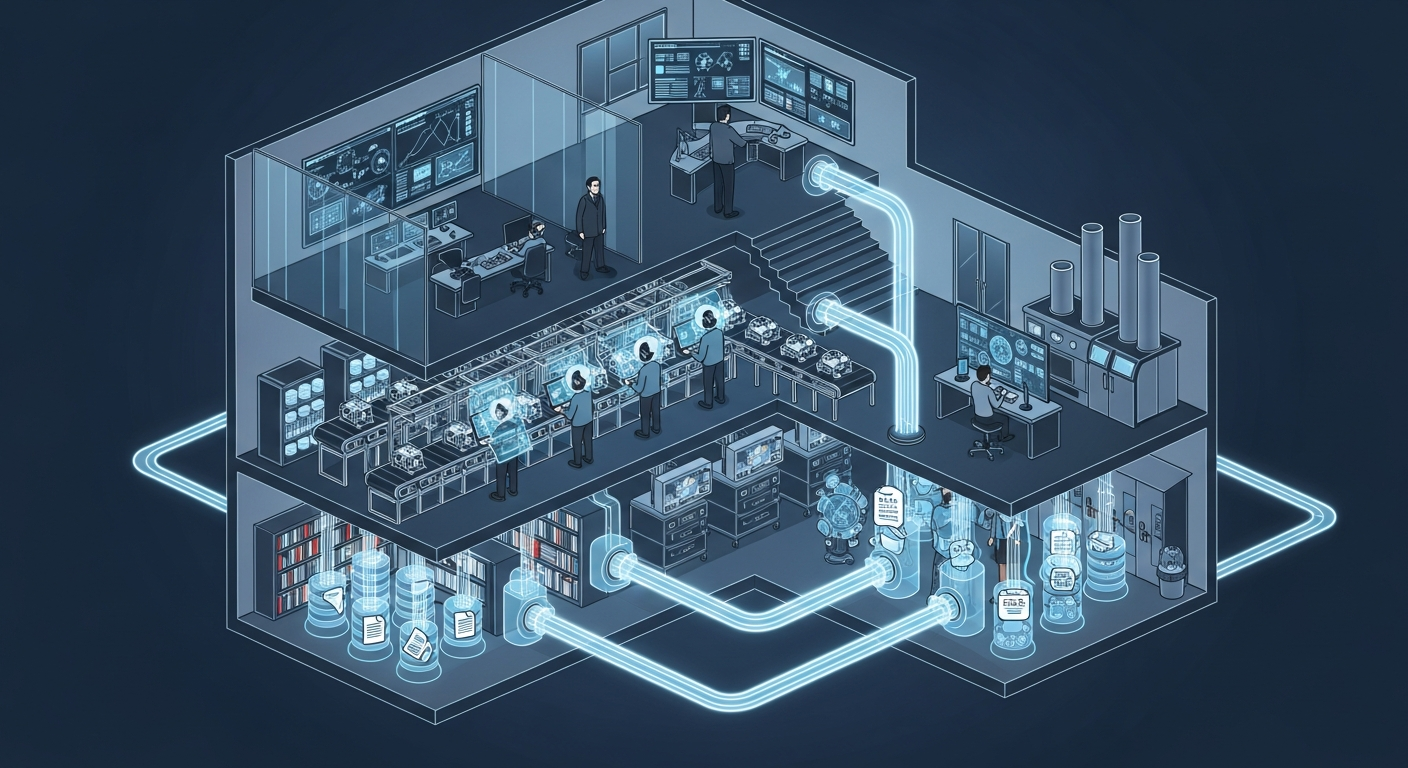
공장의 뇌는 어떻게 생겼는가 — 제조운영 AI 아키텍처 해부
지식관리, 업무자동화, 의사결정지원 — 따로 보면 다 있던 것들입니다. 제조 AI의 진짜 차이는 이 셋이 순환하면서 '우리 공장만의 지능'을 만든다는 데 있습니다.
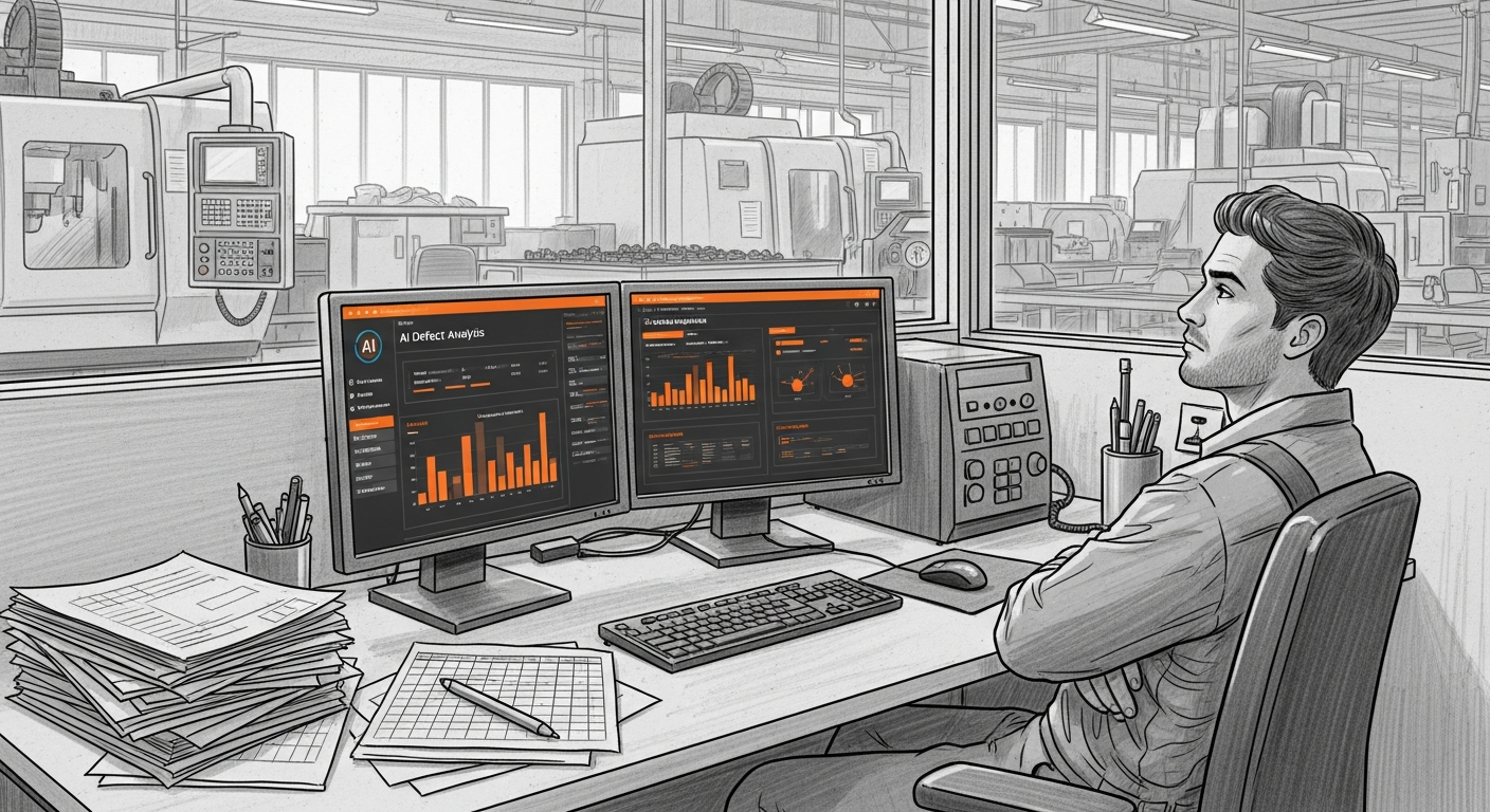
그 30분을 18년 동안 매일 반복했습니다 — 품질팀장이 본 AI Agent
18년차 품질팀장이 매일 아침 30분씩 반복하던 데이터 분석을 AI Agent가 3분 만에 해냈습니다. 챗봇과는 완전히 다른 물건 — 직접 시스템에 접근해서 데이터를 꺼내고 분석하는 AI의 현장 도입기.
Want to apply this in your factory?
MOAI helps manufacturing companies adopt AI tailored to their operations.
Talk to us →